Hypothesis Testing with Spielberg and Burton

Aim: Exploring whether the mean IMDB rating for Steven Spielberg and Tim Burton is different via Hypothesis Testing. (Language: R)

H0 = there is no difference between the mean IMBD ratings of Steven Spielberg and Tim Burton
H1 = there is a difference between the mean IMBD ratings of Steven Spielberg and Tim Burton

First we need to load the data and take a look at its contents.

movies <- read_csv(here::here("data", "movies.csv"))

## Rows: 2961 Columns: 11

## ── Column specification ────────────────────────────────────────────────────────
## Delimiter: ","
## chr (3): title, genre, director
## dbl (8): year, duration, gross, budget, cast_facebook_likes, votes, reviews,...

## 
## ℹ Use `spec()` to retrieve the full column specification for this data.
## ℹ Specify the column types or set `show_col_types = FALSE` to quiet this message.

glimpse(movies) 

## Rows: 2,961
## Columns: 11
## $ title               <chr> "Avatar", "Titanic", "Jurassic World", "The Avenge…
## $ genre               <chr> "Action", "Drama", "Action", "Action", "Action", "…
## $ director            <chr> "James Cameron", "James Cameron", "Colin Trevorrow…
## $ year                <dbl> 2009, 1997, 2015, 2012, 2008, 1999, 1977, 2015, 20…
## $ duration            <dbl> 178, 194, 124, 173, 152, 136, 125, 141, 164, 93, 1…
## $ gross               <dbl> 760505847, 658672302, 652177271, 623279547, 533316…
## $ budget              <dbl> 2.37e+08, 2.00e+08, 1.50e+08, 2.20e+08, 1.85e+08, …
## $ cast_facebook_likes <dbl> 4834, 45223, 8458, 87697, 57802, 37723, 13485, 920…
## $ votes               <dbl> 886204, 793059, 418214, 995415, 1676169, 534658, 9…
## $ reviews             <dbl> 3777, 2843, 1934, 2425, 5312, 3917, 1752, 1752, 35…
## $ rating              <dbl> 7.9, 7.7, 7.0, 8.1, 9.0, 6.5, 8.7, 7.5, 8.5, 7.2, …

Basic initial analysis to see how the mean ratings compare:

#initial observation table:
 movies %>% 
  filter(director %in% c("Steven Spielberg", "Tim Burton")) %>% 
  group_by(director) %>% 
  summarise(n = n(),
            mean = mean(rating),
            sd = sd(rating))  

## # A tibble: 2 × 4
##   director             n  mean    sd
##   <chr>            <int> <dbl> <dbl>
## 1 Steven Spielberg    23  7.57 0.695
## 2 Tim Burton          16  6.93 0.749

Comparing confidence intervals:

#creating a confidence interval
compare <- movies %>% 
  filter(director %in% c("Tim Burton", "Steven Spielberg"))   %>% 
  group_by(director) %>% 
   summarise(mean = round(mean(rating), 2),
              n = count(director),
              sd = sd(rating),
              t_critical = qt(0.975, n - 1),  #calculates the t-critical
              se = sd / sqrt(n),
              margin_of_error = t_critical * se,
              low_CI= round(mean - margin_of_error, 2) ,
              high_CI= round(mean + margin_of_error, 2)
              )%>%
  mutate(director = factor(director, levels = c("Tim Burton","Steven Spielberg")))

#graphing the confidence intervals
graph <- ggplot(compare, aes(colour=director)) +
  geom_errorbar(aes(xmin = low_CI, xmax = high_CI, y= director), width = 0.1, size = 1.5)  +
  scale_color_manual(values = c("skyblue","tomato"))+
  geom_point(aes(x=mean, y=director), size = 3 ) +
  labs(title="Do Spielberg and Burton have the same IMDB ratings?",
       subtitle="95% confidence intervals overlap",
       x="Mean IMDB Rating",
       y =" ") +
  geom_text(aes(label = low_CI, x=low_CI, y=director), size = 4, color="black", hjust = 1, vjust = 0, nudge_x = 0.05, nudge_y = 0.08) +
  geom_text(aes(label = high_CI, x=high_CI, y=director),size = 4, color="black", hjust = 1, vjust = 0, nudge_x = 0.05, nudge_y = 0.08) +
  geom_text(aes(label = mean, mean, y=director), size = 6, color="black", hjust = 1, vjust = 0, nudge_x = 0.05, nudge_y = 0.08)+
geom_rect( mapping=aes(xmin= 7.27, xmax= 7.33, ymin=0, ymax=3), color="lightgrey", alpha=0.2) +
  theme_bw()
  
  
graph +theme(legend.position = "none")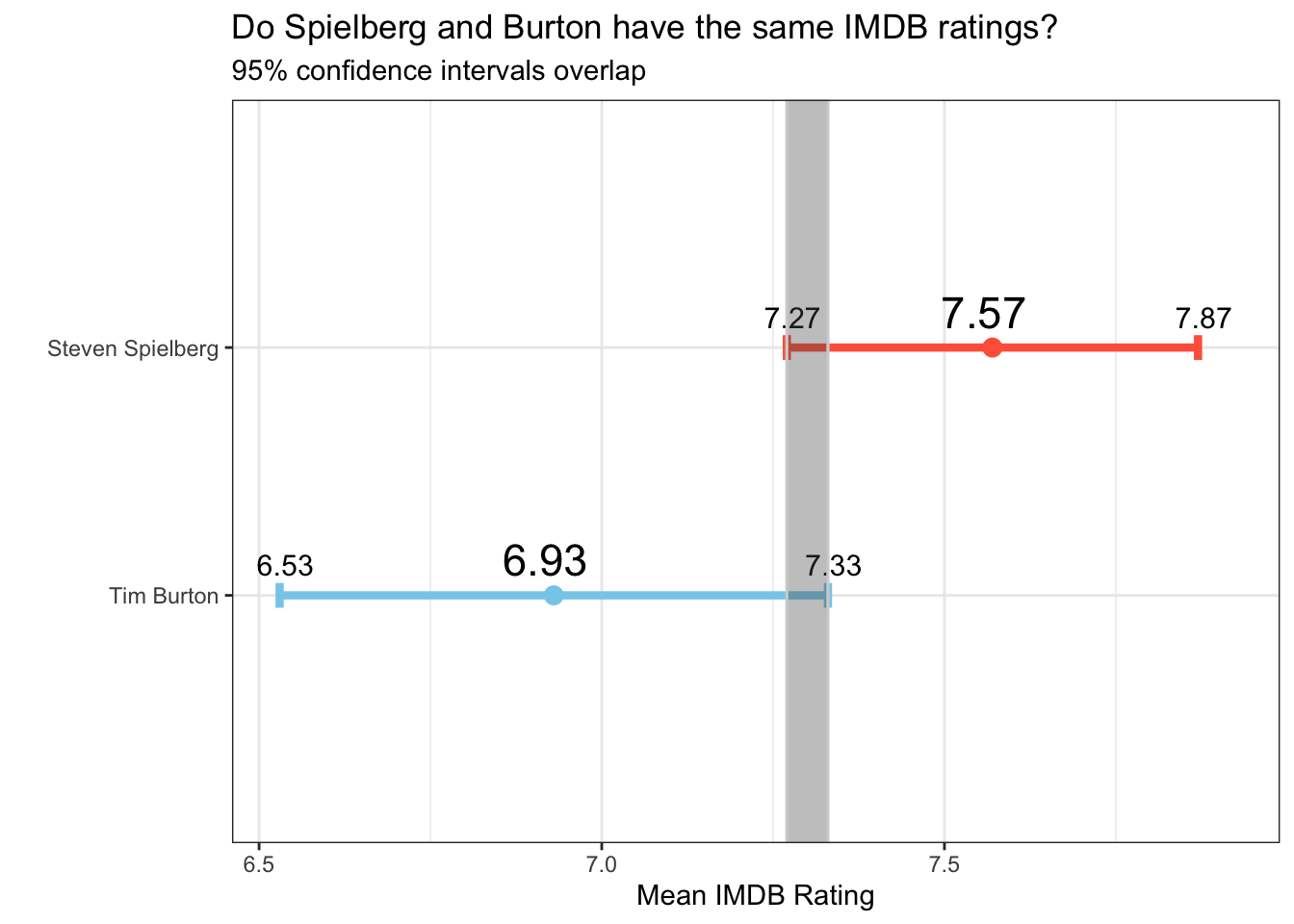 

T-test

compare2 <- movies %>% 
  filter(director %in% c("Steven Spielberg", "Tim Burton")) 

t.test(rating ~ director, data = compare2)

## 
##  Welch Two Sample t-test
## 
## data:  rating by director
## t = 2.7144, df = 30.812, p-value = 0.01078
## alternative hypothesis: true difference in means between group Steven Spielberg and group Tim Burton is not equal to 0
## 95 percent confidence interval:
##  0.1596624 1.1256637
## sample estimates:
## mean in group Steven Spielberg       mean in group Tim Burton 
##                       7.573913                       6.931250

Hypothesis testing

set.seed(1234)

obs_diff <- compare2 %>%
  specify(rating ~ director) %>%
  calculate(stat = "diff in means", order = c("Steven Spielberg", "Tim Burton"))

obs_diff

## Response: rating (numeric)
## Explanatory: director (factor)
## # A tibble: 1 × 1
##    stat
##   <dbl>
## 1 0.643

#hypothesis testing with infer:

  null_dist_movies <- compare2 %>%
  # specify variables
  specify(rating ~ director) %>%
  
  # assume independence, i.e, there is no difference
  hypothesize(null = "independence") %>%
  
  # generate 1000 reps, of type "permute"
  generate(reps = 1000, type = "permute") %>%
  
  # calculate statistic of difference, namely "diff in means"
  calculate(stat = "diff in means", order = c("Steven Spielberg", "Tim Burton"))
  
#visualise the null distribution 
null_dist_movies %>% visualize() +
  shade_p_value(obs_stat = obs_diff, direction = "two-sided")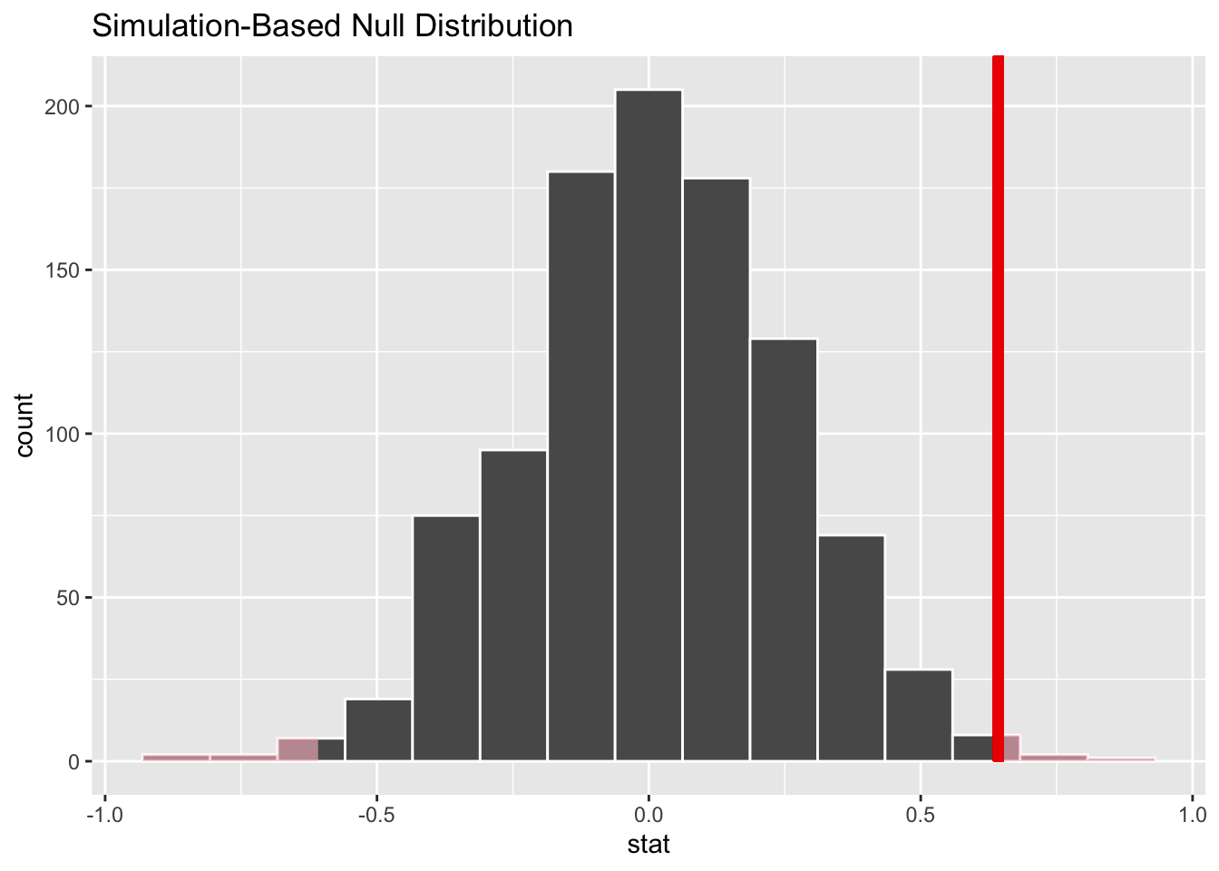

null_dist_movies %>%
  get_p_value(obs_stat = obs_diff, direction = "two_sided")

## # A tibble: 1 × 1
##   p_value
##     <dbl>
## 1   0.008

null_dist_movies %>%
  get_p_value(obs_stat = obs_diff, direction = "two_sided")

## # A tibble: 1 × 1
##   p_value
##     <dbl>
## 1   0.008