Youth Risk Behavior Surveillance

Aim:to analyse the health patterns of American high scholers (9th through 12th grade) using R libraries.

Data: Every two years, the Centers for Disease Control and Prevention conduct the Youth Risk Behavior Surveillance System (YRBSS) survey, where it takes data from high schoolers (9th through 12th grade), to analyze health patterns.

Loading the data

This data is part of the openintro textbook and we can load and inspect it.

?yrbss

data(yrbss)
glimpse(yrbss)

## Rows: 13,583
## Columns: 13
## $ age                      <int> 14, 14, 15, 15, 15, 15, 15, 14, 15, 15, 15, 1…
## $ gender                   <chr> "female", "female", "female", "female", "fema…
## $ grade                    <chr> "9", "9", "9", "9", "9", "9", "9", "9", "9", …
## $ hispanic                 <chr> "not", "not", "hispanic", "not", "not", "not"…
## $ race                     <chr> "Black or African American", "Black or Africa…
## $ height                   <dbl> NA, NA, 1.73, 1.60, 1.50, 1.57, 1.65, 1.88, 1…
## $ weight                   <dbl> NA, NA, 84.37, 55.79, 46.72, 67.13, 131.54, 7…
## $ helmet_12m               <chr> "never", "never", "never", "never", "did not …
## $ text_while_driving_30d   <chr> "0", NA, "30", "0", "did not drive", "did not…
## $ physically_active_7d     <int> 4, 2, 7, 0, 2, 1, 4, 4, 5, 0, 0, 0, 4, 7, 7, …
## $ hours_tv_per_school_day  <chr> "5+", "5+", "5+", "2", "3", "5+", "5+", "5+",…
## $ strength_training_7d     <int> 0, 0, 0, 0, 1, 0, 2, 0, 3, 0, 3, 0, 0, 7, 7, …
## $ school_night_hours_sleep <chr> "8", "6", "<5", "6", "9", "8", "9", "6", "<5"…

yrbss %>% mutate(race = factor(race))

## # A tibble: 13,583 × 13
##      age gender grade hispanic race    height weight helmet_12m text_while_driv…
##    <int> <chr>  <chr> <chr>    <fct>    <dbl>  <dbl> <chr>      <chr>           
##  1    14 female 9     not      Black …  NA      NA   never      0               
##  2    14 female 9     not      Black …  NA      NA   never      <NA>            
##  3    15 female 9     hispanic Native…   1.73   84.4 never      30              
##  4    15 female 9     not      Black …   1.6    55.8 never      0               
##  5    15 female 9     not      Black …   1.5    46.7 did not r… did not drive   
##  6    15 female 9     not      Black …   1.57   67.1 did not r… did not drive   
##  7    15 female 9     not      Black …   1.65  132.  did not r… <NA>            
##  8    14 male   9     not      Black …   1.88   71.2 never      <NA>            
##  9    15 male   9     not      Black …   1.75   63.5 never      <NA>            
## 10    15 male   10    not      Black …   1.37   97.1 did not r… <NA>            
## # … with 13,573 more rows, and 4 more variables: physically_active_7d <int>,
## #   hours_tv_per_school_day <chr>, strength_training_7d <int>,
## #   school_night_hours_sleep <chr>

skimr::skim(yrbss) #to get a feel about the dataset

Table 1: Data summary
Name	yrbss
Number of rows	13583
Number of columns	13
_______________________
Column type frequency:
character	8
numeric	5
________________________
Group variables	None

Variable type: character

skim_variable	n_missing	complete_rate	min	max	n_unique
gender	12	1.00	4	6	2
grade	79	0.99	1	5	5
hispanic	231	0.98	3	8	2
race	2805	0.79	5	41	5
helmet_12m	311	0.98	5	12	6
text_while_driving_30d	918	0.93	1	13	8
hours_tv_per_school_day	338	0.98	1	12	7
school_night_hours_sleep	1248	0.91	1	3	7

Variable type: numeric

skim_variable	n_missing	complete_rate	mean	sd	p0	p25	p50	p75	p100	hist
age	77	0.99	16.16	1.26	12.00	15.00	16.00	17.00	18.00	▁▂▅▅▇
height	1004	0.93	1.69	0.10	1.27	1.60	1.68	1.78	2.11	▁▅▇▃▁
weight	1004	0.93	67.91	16.90	29.94	56.25	64.41	76.20	180.99	▆▇▂▁▁
physically_active_7d	273	0.98	3.90	2.56	0.00	2.00	4.00	7.00	7.00	▆▂▅▃▇
strength_training_7d	1176	0.91	2.95	2.58	0.00	0.00	3.00	5.00	7.00	▇▂▅▂▅

Exploratory Data Analysis

Starting out by analyzing the weight of participants in kilograms.

#number of missing values in the 'weight' column:
sumna <- sum(is.na(yrbss['weight']))
print(paste0("there are " , sumna ," missing values." ))

## [1] "there are 1004 missing values."

#using mosaic's favstats
favstats(~weight, data=yrbss)

##    min    Q1 median   Q3    max    mean       sd     n missing
##  29.94 56.25  64.41 76.2 180.99 67.9065 16.89821 12579    1004

#as it is also apparent in the favstat's function output, there are 1004 missing values in the weight column. 

#histogram of the weight distribution
  ggplot(yrbss, aes(x=weight))+
  geom_histogram(bindwidth=5, color ="black", fill = "white")+
  labs (title = "Histogram of Weigth Distribution",
        y = "Count",
        x = "Weight (in kilograms)")+ 
  theme_bw()+
  geom_vline(aes(xintercept = mean(weight, na.rm = TRUE)), color="blue", linetype="dashed", size=1)+
  NULL

## Warning: Ignoring unknown parameters: bindwidth

## `stat_bin()` using `bins = 30`. Pick better value with `binwidth`.

## Warning: Removed 1004 rows containing non-finite values (stat_bin).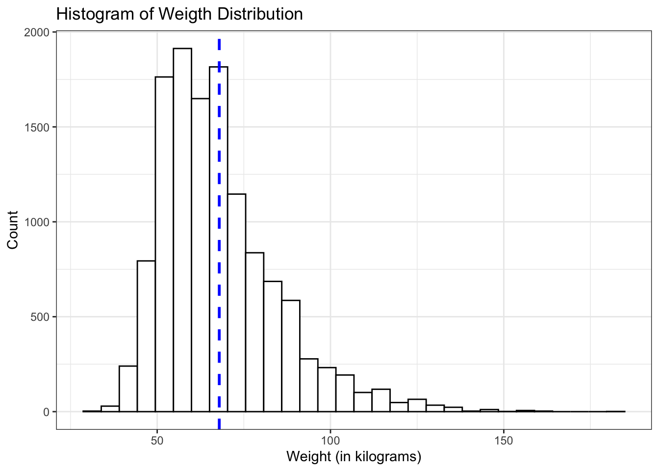

#density plot of the weight distribution
  ggplot(yrbss, aes(x=weight)) +
  geom_density() +
  labs (title = "Density Plot of Weight Distribution",
        x = "Weight (in kilograms)")+
  theme_bw()+
  NULL

## Warning: Removed 1004 rows containing non-finite values (stat_density).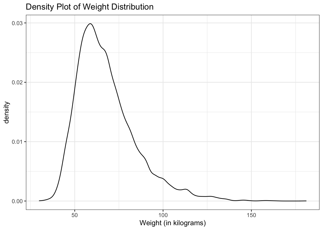

Is there a relationship between a high schooler’s weight and their physical activity? By adding a new column that shows whether a student exercised more than 3 days a week or not, the relationship with exercises and non-exercises can be easily determined.

yrbss %>%
  filter(!is.na(physically_active_7d))%>%
  ggplot(aes(x = factor(physically_active_7d))) +
  geom_boxplot(aes(y=weight))+
  labs (title = "Distribution of Weight by Number of Active days in a week",
        x = "Number of Active Days in a Week",
        y = "weight (kg)") +
  theme_bw()

## Warning: Removed 946 rows containing non-finite values (stat_boxplot).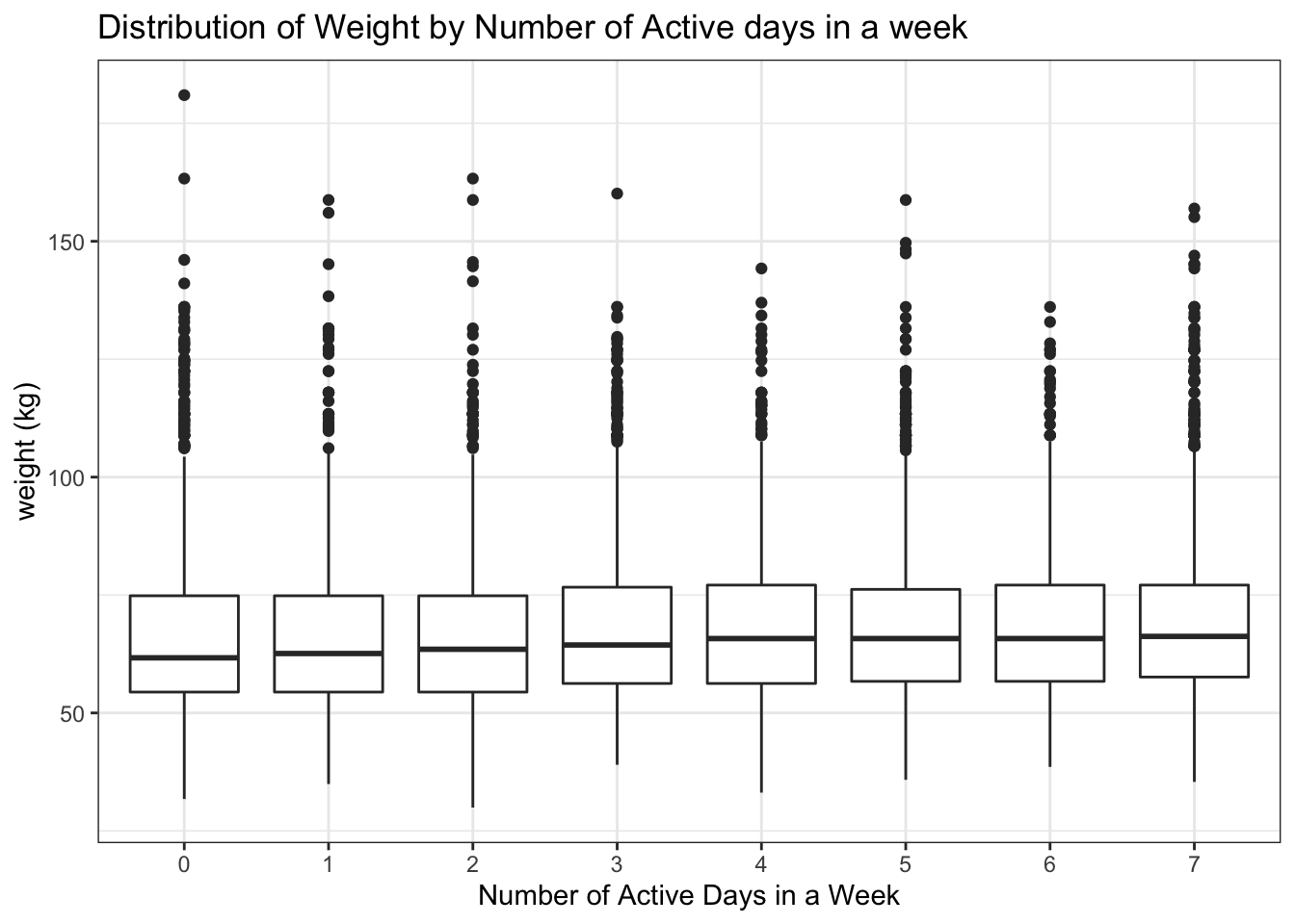

  #adding the new variable `physical_3plus` that shows if a student is physically active 3 or more days a week. 
  physical <- yrbss %>% 
    mutate(physical_3plus = case_when(physically_active_7d >= 3 ~ "yes",
                                       physically_active_7d < 3 ~ "no"),
          physical_3plus = factor(physical_3plus, levels = c("yes", "no")))  
 
 count_physical <- physical %>% 
   filter(!is.na(physical_3plus)) %>% 
   count(physical_3plus) %>% 
   mutate(prop = n/sum(n))
 
 #5685, 2656 
 
 prop.test(count_physical$n[2]  , count_physical$n[2] + count_physical$n[1])

## 
##  1-sample proportions test with continuity correction
## 
## data:  [ out of +count_physical$n out of count_physical$n[2]2 out of count_physical$n[1]
## X-squared = 1522.1, df = 1, p-value < 2.2e-16
## alternative hypothesis: true p is not equal to 0.5
## 95 percent confidence interval:
##  0.3228978 0.3389583
## sample estimates:
##        p 
## 0.330879

95% confidence interval for the population proportion of high schools that are NOT active 3 or more days per week?

The 95 percent confidence interval according to the prop.test function is from 0.3228978 to 0.3389583.

data: [ out of +count_physical$n out of count_physical$n[2]2 out of count_physical$n[1] X-squared = 1522, df = 1, p-value <2e-16 alternative hypothesis: true p is not equal to 0.5 95 percent confidence interval: 0.323 0.339 sample estimates: p 0.331

Initial plotting of the data doesn’t suggest a strong correlation between weekly physical activity levels and weight.

A boxplot of physical_3plus vs. weight. Is there a relationship between these two variables?

#removing rows that contain NAs from the physical table... 
   physical <- physical %>% 
   filter(!is.na(physical_3plus) & !is.na(weight))
   
#box plot of physical_3plus vs weight:
  
  ggplot(physical, aes(x=physical_3plus, y = weight)) +
  geom_boxplot()+
  labs (title = "Distribution of Weight, Based on weekly activity level",
        x = "Working out 3 or more days: Yes or No",
        y = "weight (kg)") +
  theme_bw()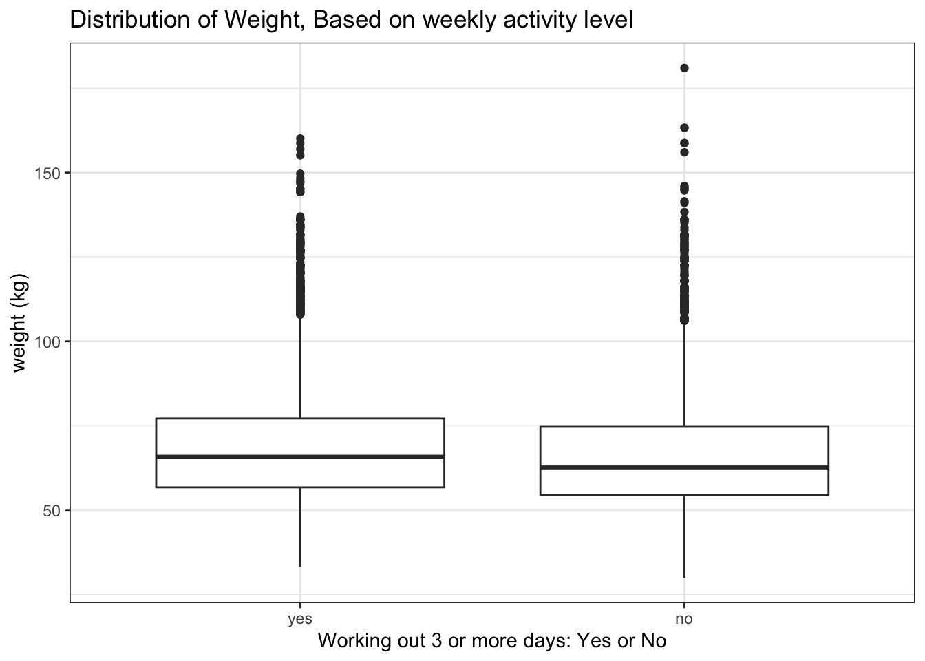

People who work out 3 days a week or more are slightly heavier on average. One might expect the opposite, but weight is not a great indicator of fitness levels as it varries widely with height, and the number of workout days might not indicate the intensity of the workouts either. We would expect a stronger negative correlation between bodyfat percentage and number of active days a week.

Confidence Interval

Boxplots show how the medians of the two distributions compare, but we can also compare the means of the distributions using either a confidence interval or a hypothesis test. Note that when we calculate the mean, SD, etc. weight in these groups using the mean function, we must ignore any missing values by setting the na.rm = TRUE.

set.seed(1234)
#calculating CI using formulas:

#physical_3plus == "yes
 yes_result<- physical %>% 
   filter(physical_3plus == "yes") %>% 
   summarise( yes_mean = mean(weight, na.rm = TRUE),
              yes_n = count(physical_3plus == "yes"),
              yes_sd = sd(weight, na.rm = TRUE),
              t_critical = qt(0.975, yes_n -1),
              se_yes = yes_sd / sqrt(yes_n),
              margin_of_error = t_critical * se_yes,
              yes_low_CI= yes_mean - margin_of_error,
              yes_high_CI= yes_mean + margin_of_error
              )

print(paste0("the confidence interval is ",  as.numeric(yes_result['yes_low_CI']), " - ", as.numeric(yes_result['yes_high_CI']) ))

## [1] "the confidence interval is 68.094807893518 - 68.8021328880692"

#we can get a very similar result using the bootstrap approach for confidence intervals by infer package:

boot_dist1 <- physical %>% 
   filter(physical_3plus == "yes") %>% 

  specify(response = weight) %>%
  # Generate bootstrap samples
  generate(reps = 1000, type = "bootstrap") %>%
  # Calculate mean of each bootstrap sample
  calculate(stat = "mean")

boot_dist1

## Response: weight (numeric)
## # A tibble: 1,000 × 2
##    replicate  stat
##        <int> <dbl>
##  1         1  68.2
##  2         2  68.3
##  3         3  68.4
##  4         4  68.4
##  5         5  68.8
##  6         6  68.0
##  7         7  68.5
##  8         8  68.4
##  9         9  68.6
## 10        10  68.6
## # … with 990 more rows

percentile_ci1 <- get_ci(boot_dist1, level = 0.95, type ="percentile") 

#visualisation of the resulting bootstrap distribution and the CIs
  visualize(boot_dist1) +
  shade_ci(endpoints=percentile_ci1, fill="khaki") +
  geom_vline(xintercept = yes_result$yes_low_CI, colour ="red") +
  geom_vline(xintercept = yes_result$yes_high_CI, colour = "red") +
  NULL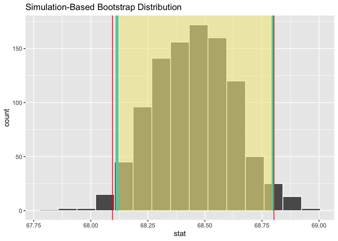

#physical_3plus == "no"
no_result <-physical %>% 
   filter(!is.na(physical_3plus)) %>%
   filter(physical_3plus == "no") %>% 
   summarise( no_mean = mean(weight, na.rm = TRUE),
              no_n = count(physical_3plus == "no"),
              no_sd = sd(weight, na.rm = TRUE),
              t_critical = qt(0.975, no_n -1),
              se_no= no_sd / sqrt(no_n),
              margin_of_error = t_critical * se_no,
              no_low_CI= no_mean - margin_of_error,
              no_high_CI= no_mean + margin_of_error)

print(paste0("the confidence interval is ",  as.numeric(no_result['no_low_CI']), " - ", as.numeric(no_result['no_high_CI']) ))

## [1] "the confidence interval is 66.1286201312585 - 67.2191521213521"

#we can also get a very similar result using the bootstrap approach for confidence intervals by infer package:

boot_dist2 <- physical %>% 
   filter(!is.na(physical_3plus)) %>% 
   filter(physical_3plus == "no") %>% 
   specify(response = weight) %>%
  # Generate bootstrap samples
  generate(reps = 1000, type = "bootstrap") %>%
  # Calculate mean of each bootstrap sample
  calculate(stat = "mean")

percentile_ci <- get_ci(boot_dist2, level = 0.95, type ="percentile") 

#visualisation of the resulting bootstrap distribution and the CIs
  visualize(boot_dist2) +
  shade_ci(endpoints=percentile_ci, fill="khaki") +
  geom_vline(xintercept = no_result$no_low_CI, colour ="red") +
  geom_vline(xintercept = no_result$no_high_CI, colour = "red") +
  labs(title="Simulation-Based Bootsrap Distribution for No Answers") +
  NULL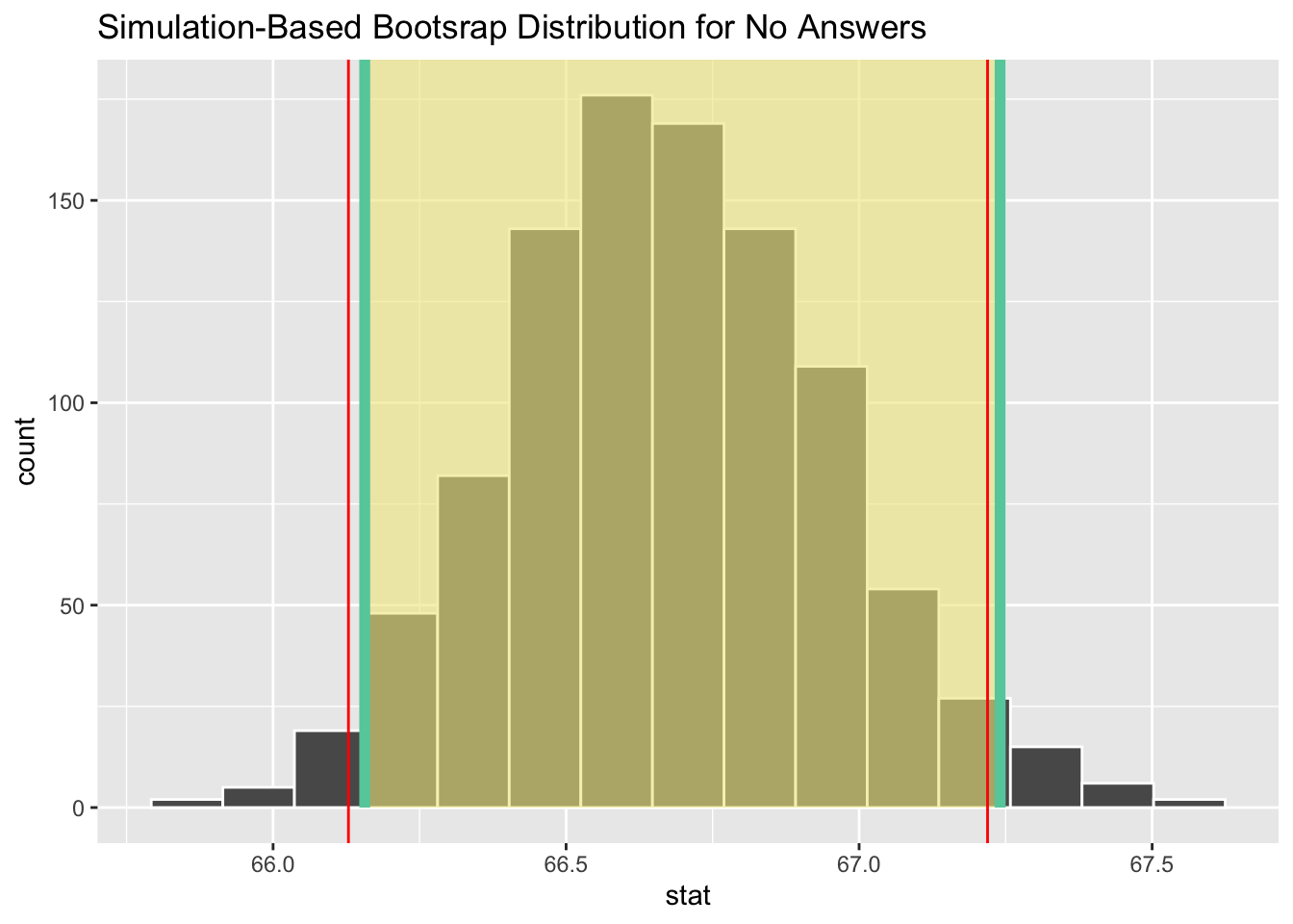

There is an observed difference of about 1.77kg (68.44 - 66.67), and we notice that the two confidence intervals do not overlap. It seems that the difference is at least 95% statistically significant. Let us also conduct a hypothesis test.

Hypothesis test with formula

Null and alternative hypothesis: H0 = there is no difference in the weight of those who exercise 3 times a week and more compared to those who do not. H1 = there is a difference in the weight of those who exercise 3 times a week and more and those who do not.

t.test(weight ~ physical_3plus, data = physical)

## 
##  Welch Two Sample t-test
## 
## data:  weight by physical_3plus
## t = 5.353, df = 7478.8, p-value = 8.908e-08
## alternative hypothesis: true difference in means between group yes and group no is not equal to 0
## 95 percent confidence interval:
##  1.124728 2.424441
## sample estimates:
## mean in group yes  mean in group no 
##          68.44847          66.67389

Since the T value is 5 we can reject the NULL hypothesis, which means that we statistically sufficient evidence to say that there is a difference in the mean weight of those who work out more than 3 days a week and those who don’t.

Hypothesis test with `infer` package

obs_diff <- physical %>%
  specify(weight ~ physical_3plus) %>%
  calculate(stat = "diff in means", order = c("yes", "no"))

obs_diff

## Response: weight (numeric)
## Explanatory: physical_3plus (factor)
## # A tibble: 1 × 1
##    stat
##   <dbl>
## 1  1.77

Simulating the test on the null distribution, which we will save as null.

  null_dist <- physical %>%
  # specify variables
  specify(weight ~ physical_3plus) %>%
  
  # assume independence, i.e, there is no difference
  hypothesize(null = "independence") %>%
  
  # generate 1000 reps, of type "permute"
  generate(reps = 1000, type = "permute") %>%
  
  # calculate statistic of difference, namely "diff in means"
  calculate(stat = "diff in means", order = c("yes", "no"))

We can visualize this null distribution with the following code:

ggplot(data = null_dist, aes(x = stat)) +
  geom_histogram()

## `stat_bin()` using `bins = 30`. Pick better value with `binwidth`.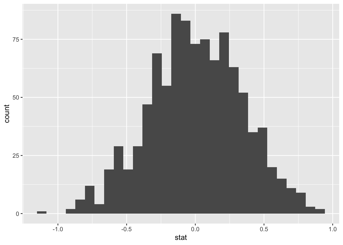

The p-value for your hypothesis test using the function infer::get_p_value().

null_dist %>% visualize() +
  shade_p_value(obs_stat = obs_diff, direction = "two-sided")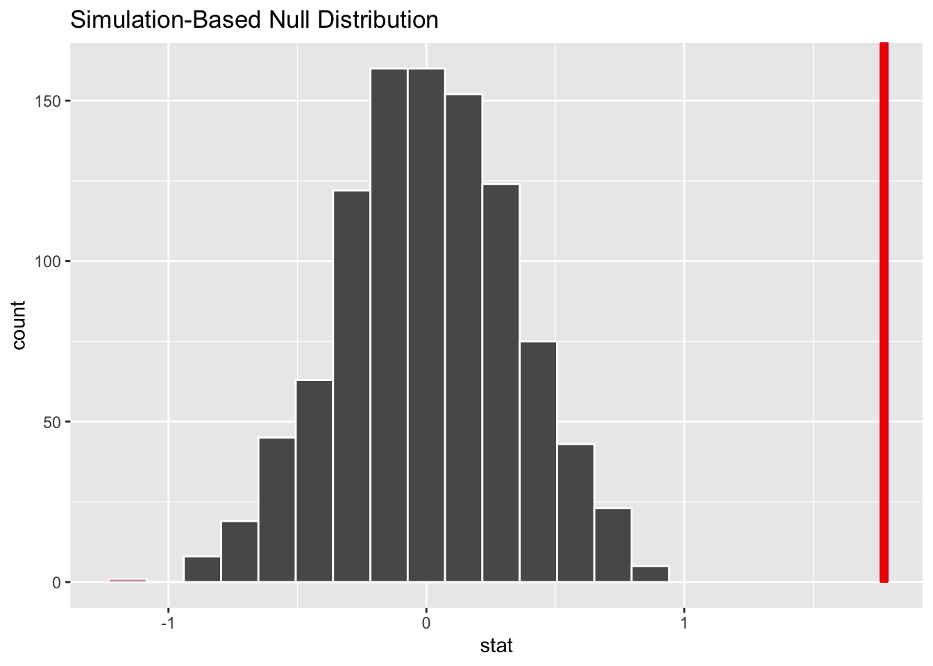

null_dist %>%
  get_p_value(obs_stat = obs_diff, direction = "two_sided")

## Warning: Please be cautious in reporting a p-value of 0. This result is an
## approximation based on the number of `reps` chosen in the `generate()` step. See
## `?get_p_value()` for more information.

## # A tibble: 1 × 1
##   p_value
##     <dbl>
## 1       0

Conclusion